Last week, I finally completed the full extent of my model architecture! We have now incorporated most of the data that we will use in our final model, multiple layers of prediction using an elastic net regression with optimized parameters, and model ensembling. Three items are on our agenda for this week. First, I will fix a few lingering errors that I noticed in last week’s model. Then, I will build a visualization for my 2024 election predictions. And finally, I will attempt to implement a Monte Carlo simulation that tests the uncertainty of my model.
Error Correction
I noticed two errors in my previous model. First, last week, I incorrectly assumed that the ensemble learning weights do not have to sum to one. Turns out, I misinterpreted super learning as an unconstrained optimization problem. In fact, the idea is to take a convex combination of each base model and produce a single prediction, which means that the weights actually do have to add to one. In this week’s model, I add that constraint.
Second, I may need to modify my method for imputing missing data. Currently, there are many indicators — both polls and economic indicators — that do not extend as far back in time as my output variable. However, in previous models, I thought it would be remiss to forego a few extra years of training simply because a few indicators are missing. In fact, there is so much data missing, that if I threw out every state or every year in which an indicator was missing, I would end up with hardly any training data at all! Because there is so much missing data, it is also not impossible to impute. After all, I can’t just invent polling data for an entire year!
So, what I have done in previous weeks is to simply impute the missing indicators as zero. That way, when I train the model, the coefficients on the missing indicators will not effect the coefficients of the non-missing indicators. However, this approach, while plausible, could potentially bias the coefficients of both indicators themselves. (Here, when I say “missing” indicators, I am referring indicators for which data during some subset of the years from 1952 to 2022 are missing.) For example, suppose poll_margin_nat_7 — the indicator for the national polling margin seven weeks before the election — is missing from the years 1952 to 2000, and accurate from 2000 to 2020. Then, the coefficient of the polling variable is likely biased downward because, for the earlier period, I have assumed that polling had no effect on the vote margin (when in reality, it likely did). Similarly, the other variables are likely biased upwards, because they could be picking up some of the variation that should have been explained by polling.
Unfortunately, this issue isn’t easy to solve. I can minimize the bias by excluding years with lots of missing indicators from my dataset, but that reduces that already-small sample I have to train on, which could cause overfitting and make both my in-sample and out-of-sample predictions less accurate. To be rigorous about this, let’s define a precise “overfitting” metric as the differential between the out-of-sample mean squared error of a given model and some function of the in-sample mean squared error of that model.
If the model is correctly specified, it can be shown under mild assumptions that the expected value of the MSE for the training set (i.e. our in-sample MSE) is (n − p − 1)/(n + p + 1) < 1 times the expected value of the MSE for the validation set (i.e. our out-of-sample MSE), where n is the number of observations, and p is the number of features. Luckily,it is possible to directly compute the factor (n − p − 1)/(n + p + 1) by which the training MSE underestimates the validation MSE. So, we can create our “overfitted” metric as:
$$ \mathrm{overfit} = \mathrm{MSE\_out} - \left(\frac{n + p + 1}{n − p − 1}\right) \mathrm{MSE\_in} $$The following table reports the overfitting metric for each of three potential subsets of the data:
# Define formulas
state_formula <- as.formula(paste("pl ~ pl_lag1 + pl_lag2 + hsa_adjustment +",
                                  "rsa_adjustment + elasticity +",
                                  "cpr_solid_d + cpr_likely_d	+ cpr_lean_d +",
                                  "cpr_toss_up + cpr_lean_r + cpr_likely_r	+ cpr_solid_r + ",
                                  paste0("poll_lean_", 7:36, collapse = " + ")))

nat_fund_formula <- as.formula("margin_nat ~ incumb_party:(jobs_agg +
                                     pce_agg + rdpi_agg + cpi_agg + ics_agg +
                                     sp500_agg + unemp_agg)")

nat_polls_formula <- as.formula(paste("margin_nat ~ incumb_party:(weighted_avg_approval) + ",
                                           paste0("poll_margin_nat_", 7:36, collapse = " + ")))

# create lists of dataframes for comparison
df_subset_1972 <- df %>% filter(year >= 1972)
df_subset_1980 <- df %>% filter(year >= 1980)
df_subset_2000 <- df %>% filter(year >= 2000)
dfs <-  list(df, df_subset_1972, df_subset_1980, df_subset_2000)

# Initialize a matrix to store the MSEs (3 models x 4 subsets)
mse_matrix <- matrix(nrow = 4, ncol = 3)
rownames(mse_matrix) <- c("Full Data", "Subset >= 1972", "Subset >= 1980", "Subset >= 2000")
colnames(mse_matrix) <- c("State Model", "Nat Fund Model", "Nat Polls Model")

for (i in seq_along(dfs)) {
  # access df
  df <- dfs[[i]]

  # Split data
  state_data <- split_state(df, 2024)
  national_data <- split_national(df, 2024)

  # Train models
  state_model_info <- train_elastic_net(state_data$train, state_formula)
  nat_fund_model_info <- train_elastic_net(national_data$train, nat_fund_formula)
  nat_polls_model_info <- train_elastic_net(national_data$train, nat_polls_formula)

  # Store MSEs in the matrix
  mse_matrix[i, 1] <- calculate_overfit(state_model_info$out_of_sample_mse, state_model_info$in_sample_mse,
                                        state_model_info$n, state_model_info$p)
  mse_matrix[i, 2] <- calculate_overfit(nat_fund_model_info$out_of_sample_mse, nat_fund_model_info$in_sample_mse,
                                        nat_fund_model_info$n, nat_fund_model_info$p)
  mse_matrix[i, 3] <- calculate_overfit(nat_polls_model_info$out_of_sample_mse, nat_polls_model_info$in_sample_mse,
                                        nat_polls_model_info$n, nat_polls_model_info$p)
}

print(mse_matrix)
##                State Model Nat Fund Model Nat Polls Model
## Full Data         6.403523       7.848683    -145.1184452
## Subset >= 1972    4.333628     -21.224004    -248.5398521
## Subset >= 1980    6.019361      -9.276520      21.6290282
## Subset >= 2000   10.246393      -4.000452       0.3900102
This testing suggests that the 1972 subset is best, which is what I will use for the remainder of the blog.
Visualizing the prediction
Voila! Below, find my predicted electoral map for the 2024 election. I used an interactive hex map, visualized with plotly, using the standard coordinates for the US states and districts. There are still some issues with this prediction. For one, the prediction for Washington D.C. says that the Democrats will win approximately 104 percent of the vote share. Now, I’m from D.C. — and trust me: we vote very blue. But I know for a fact that there’s no way the Democrats win 104 percent of our residents! Something is clearly wrong, likely because my outcome variable is not bounded. This will be fixed in future blog iterations.
# Define formulas
state_formula <- as.formula(paste("pl ~ pl_lag1 + pl_lag2 + hsa_adjustment +",
                                  "rsa_adjustment + elasticity +",
                                  "cpr_solid_d + cpr_likely_d	+ cpr_lean_d +",
                                  "cpr_toss_up + cpr_lean_r + cpr_likely_r	+ cpr_solid_r + ",
                                  paste0("poll_lean_", 7:36, collapse = " + ")))

nat_fund_formula <- as.formula("margin_nat ~ incumb_party:(jobs_agg +
                                     pce_agg + rdpi_agg + cpi_agg + ics_agg +
                                     sp500_agg + unemp_agg)")

nat_polls_formula <- as.formula(paste("margin_nat ~ incumb_party:(weighted_avg_approval) + ",
                                           paste0("poll_margin_nat_", 7:36, collapse = " + ")))

# Split data, using the 1972 subset
state_data <- split_state(df_subset_1972, 2024)
national_data <- split_national(df_subset_1972, 2024)

# Train models
state_model_info <- train_elastic_net(state_data$train, state_formula)
nat_fund_model_info <- train_elastic_net(national_data$train, nat_fund_formula)
nat_polls_model_info <- train_elastic_net(national_data$train, nat_polls_formula)
ensemble <- train_ensemble(list(nat_fund_model_info, nat_polls_model_info))

# Make predictions
state_predictions <- make_prediction(state_model_info, state_data$test)
nat_fund_predictions <- make_prediction(nat_fund_model_info, national_data$test)
nat_polls_predictions <- make_prediction(nat_polls_model_info, national_data$test)
ensemble_predictions <- make_ensemble_prediction(ensemble, national_data$test)

# Create the prediction tibble
df_2024 <- tibble(
  state = state_data$test$state,
  abbr = state_data$test$abbr,
  electors = state_data$test$electors,
  partisan_lean = as.vector(state_predictions)
  ) %>%
  # filter unnecessary districts
  filter(!abbr %in% c("ME_d1", "NE_d1", "NE_d3")) %>%
  # Add national predictions - using first value since they're the same for all states
  mutate(
    margin_polls = first(as.vector(nat_polls_predictions)),
    margin_fund = first(as.vector(nat_fund_predictions)),
    margin_ensemble = first(as.vector(ensemble_predictions))
  ) %>%
  # Calculate final margins and color categories
  mutate(
    margin_final = partisan_lean + margin_ensemble,
    d_pv = margin_final + 50,
    r_pv = 100 - d_pv,
    category = case_when(
      d_pv > 60 ~ "Strong D",
      d_pv > 55 & d_pv < 60 ~ "Likely D",
      d_pv > 50 & d_pv < 55 ~ "Lean D",
      d_pv > 45 & d_pv < 50 ~ "Lean R",
      d_pv > 40 & d_pv < 45 ~ "Likely R",
      TRUE ~ "Strong R"
    ),
    # Convert color_category to factor with specific ordering
    category = factor(
      category,
      levels = c("Strong R", "Likely R", "Lean R", "Lean D", "Likely D", "Strong D")
    ),
    # calculate electors that each party wins
    d_electors = sum(ifelse(category %in% c("Lean D", "Likely D", "Strong D"), electors, 0)),
    r_electors = sum(ifelse(category %in% c("Lean R", "Likely R", "Strong R"), electors, 0))
  )

electoral_map <- create_electoral_hex_map(df_2024)
electoral_map
Clearly, this would be a very unfortunate electoral college result for Vice President Kamala Harris, as she loses almost every single swing state.
Quantifying uncertainty
To determine how uncertain my predictions are, we can run Monte Carlo simulations of the election. For the sake of simplicity for this blog post, we will only run the simulations at the state level, and we will assume the national vote margin is true. Our simulations rely on the fact that each state’s predicted vote margin is actually a normal random variable, with mean centered at the predicted value and a standard deviation of three percent. (Note: this value is arbitrary and hard-coded, but in future weeks we will find a way of endogenizing it, perhaps by using the square root of the variance in the state’s recent voting history as the standard deviation instead.)
Then, following the methodology from the Economist, we run 10,001 election simulations, recording the total number of electoral college votes each candidate wins in each simulation.
The following graph plots smoothed histograms for the electoral college votes for Harris and Trump respectively
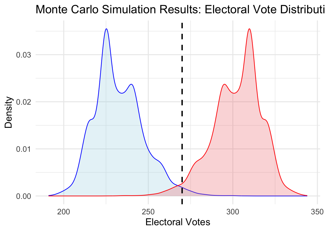 From these simulations, Harris wins approximately 1.4 percent of the time, and Trump wins approximately 97.6 percent of the time. (The remaining percent accounts for ties, when both candidates win 269 electoral votes.) Note that the curves plotting Harris’s electoral votes and Trump’s electoral votes are symmetric. This makes sense, because they must sum to 538.