Overview

Okay, something is seriously wrong with my model. Recall that my final model’s predictions involve an ensemble between the fundamentals model and the polling model. Well, this week when I ran the model, I realized that the ensemble assigned a negative weight to the fundamentals model. Admittedly it was only slightly negative, but still — that shouldn’t happen. Immediately, alarm bells went off. First of all, I modified the ensemble model from performing ordinary least squares, your classic regression, to non-negative least squares, which imposes an added restriction that all coefficients must be non-negative. I solved the optimization problem using this method. Still, though, the ensemble model shrank the fundamentals model to zero, and assigned the polls model a weight of \(1\).

Odd.

I confess, I spent a lot of time trying to find out why the fundamentals model was so bad, and I couldn’t entirely figure it out. I tried multiple different permutations of the regression specification, I tried aggregating the economic fundamentals a different way, I tried adding the base terms to the regression in addition to the cross terms. Nothing worked. Consistently, I would get \(R^2\) as low as \(0.3\), and an adjusted \(R^2\) in the negatives. The out-of-sample MSE was often over four times as large as the in-sample MSE. And worst of all, the expected sign on the coefficients were the wrong direction — somehow, real disposable personal income was a negative predictor of vote margin, not a positive one.

Perhaps I will figure out what’s up with the fundamentals in a future week. In the mean time, it doesn’t actually affect my predictions that much — the polls model seems to be quite accurate:

• \(R^2 = 0.879\)
• \(R_{\mathrm{adj}}^{2} = 0.793\)
• \(MSE_{\mathrm{out}} = 4.8\)

One nice thing about this bug is that it actually inspired me to rerun the entire model, except instead of vote margin, I used vote share. While it didn’t solve the issue with the fundamentals model, it did reveal something: the vote share model is actually more accurate than the vote margin one! Moving forward, I will be using the vote share model instead. (This also has the added benefit of inadvertently resolving my Washington D.C. vote share issue from last week.)

I also fixed two other small mistakes. First, I realized that I was calculating a state’s elasticity incorrectly. Rather than measuring it in absolute terms, I changed it to be in relative terms:

where \(s_{t}\) is the state’s vote in year \(t\) and \(n_{t}\) is the national vote in year \(t\).

Second, I noticed that my state level forecast for the partisan lead included significant coefficients for several of Cook Political Report forecasts metics. However, I had neglected to include these forecasts in the testing data, so my results were somewhat biased. All these changes came together to give me the following map of the 2024 election:

A much better result for Harris, don’t you think?

A New Simulation Method

My biggest improvement this week, however, was in the simulation process.

Simulations are used to test the uncertainty in an election prediction model. Running simulations allows me to introduce a slight variations in the values of my estimates and see just how much the election outcome changes as a result of these variations. Last week, I implemented an incredibly crude simulation approach. I assumed that the predicted national vote share was absolutely true, and that the predicted vote at the state level was the mean of a normal random variable with a standard deviation of three points.

Both of these assumptions are questionable. My prediction for the national vote share also has some degree of uncertainty, of course. Not to mention the fact that a three-point standard deviation was chosen completely arbitrarily. This week, I will introduce a new simulation process so that I avoid having to make the same assumptions I did last week.

For this simulation approach, I will introduce uncertainty in my estimates, not my predictions. This is an important distinction: the estimates refer to the vector of coefficients, \(\vec{\beta}\), that I calculated using multiple regression. The predictions, on the other hand, refer to the vector of outputs, \(\vec{\hat{y}}\), that I calculated by plugging in the 2024 values for all my predictors and computing a linear combination. I argue that varying \(\vec{\beta}\) makes more sense than varying \(\vec{\hat{y}}\), because it accounts for the fact that sampling variability makes the model’s estimates of the underlying relationships between the different variables uncertain. The coefficients could be slightly different if I had different data, so by introducing variation in \(\vec{\beta}\), I am capturing the true uncertainty in how predictors relate to the outcome.

So, I now simulate a set of coefficients by drawing from a multivariate normal distribution where the mean of each coefficient is the point estimate from the model, and the variance of each coefficient is determined by the square of its standard error. Of course, unlike with OLS regression, there is no easy closed form to get the variance of each coefficient. Instead, we have to “bootstrap” our model to calculate standard errors. Bootstrapping is a process where I draw \(n\) observations from my original dataset with replacement \(s\) different times. I will then make \(s\) different “copies” of my data. Then, I refit the model on each sample, and observe how the coefficients vary. By doing this, I can empirically estimate the variability in my coefficient estimates, and thus, the uncertainty in my election predictions.

Without further ado, here is the distribution:

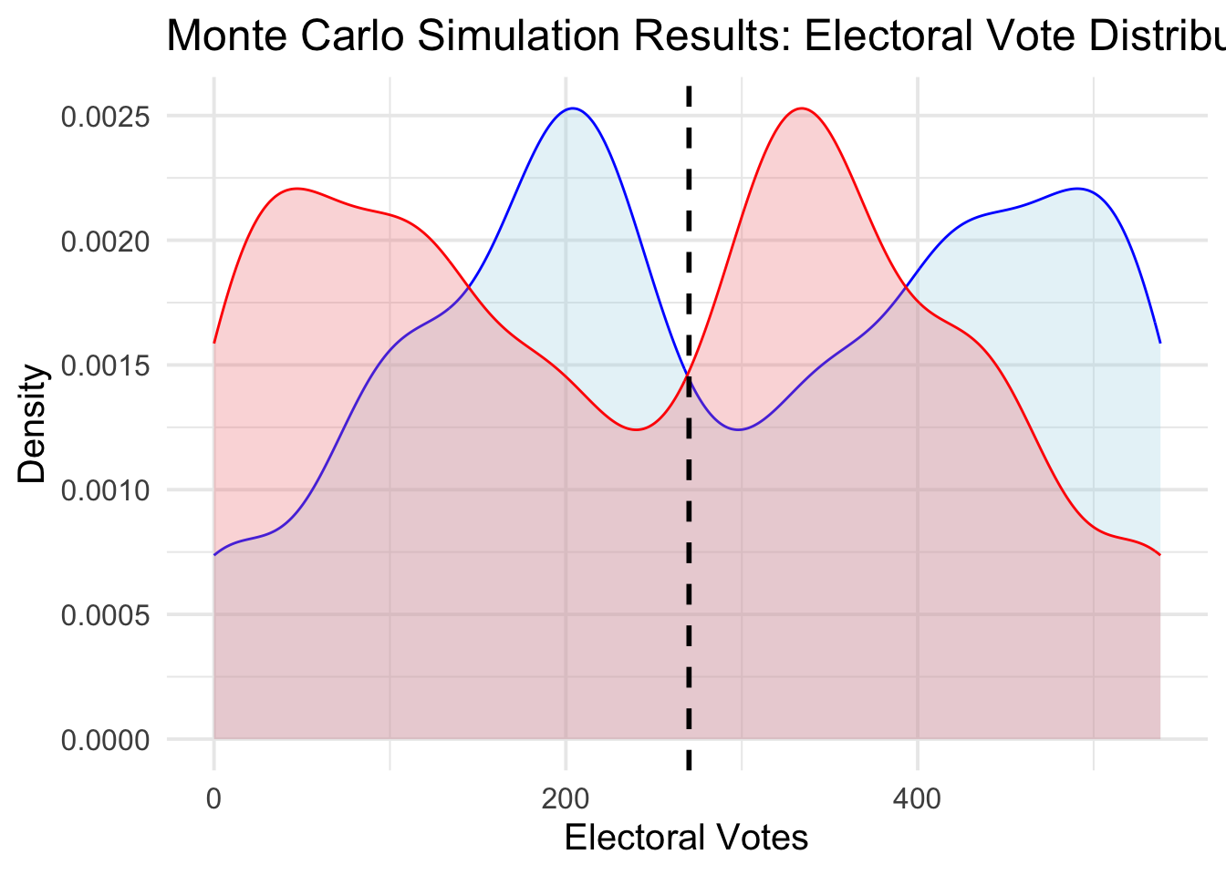
Woah. Something is definitely wrong. First of all, it is good that the Republican and Democratic electoral college votes are symmetric. But the mode of the distribution should not be all the way in the 400s. After all, my point estimate indicated that Harris wins just 287 votes — enough to win, but not a landslide. Second, the distribution is quite wonky and uninterpretable. This is a problem, considering that it makes intuitive sense for closer elections to be more likely, and distant elections to be less so.

Ultimately, beyond coding mistakes (of which I am sure there are a few), I can think of several problems with my approach. First, my code, as written, introduces variation even in coefficients that the elastic net has shrunk to zero. These don’t bias my estimates, because the normal random variable would just be centered around zero, but they do introduce extranous noise into my simulation. Second, I am varying many coefficients at once. And not all these coefficients are statistically significant, which means they sometimes have a pretty high standard error. As a result, we see large swings in electoral college results, because the slight variances all get magnified. A slightly larger \(\beta_1\) gets applied, across the board, to all 50 states (and a few districts), which can end up having huge effects.

It seems that my prior was wrong, and that, in fact, it might be better to introduce variance somewhere else in the model. Next week, I will attempt to introduce variance in the testing data.