Introduction
Simulation has become the bane of my existence. Two weeks ago, I implemented a simple simulation approach, in which I set the predicted value for each state to be the mean of a normal random variable with a standard deviation of 3 percent. Of course, the 3 percent number was entirely arbitrary, so last week, I tried a more complicated approach, where I introduced uncertainty in my estimates — the vector of coefficients \(\vec{\beta}\) — rather than the predictions themselves.
This methodology turned out to be an absolute failure — for some reason, the most common result was to for the Democrats to win something like 500 electoral votes and for the Republicans to win just 20 or 30. Ridiculous, clearly.
This week, I return to a simulation approach that involves varying the predictions themselves, rather than the estimates. However, I avoid the problem of setting a 3 percent standard deviation by attempting to come up with a good estimate for the standard error of the prediction. Much of the work this was actually math, not coding, so I thought I would show a little bit of what I have been thinking about.
Theory
When I run a Monte Carlo simulation for predicting both the national vote share and the state-level vote shares, I am essentially creating many “what-if” scenarios based on my model’s predictions. Think of the actual predictions that I compute by plugging in the 2024 predictors into the model as point estimates. They are the most likely result, but there is also some uncertainty on either side of the prediction. To quantify the spread of this uncertainty, I need to find some way to calculate the “standard error of the prediction,” otherwise known as the “forecast variance.” Let’s try to derive a reasonable result for this value. We’ll start with basic OLS regression, and then see if we can generalize to the elastic net case, which is the model that I currently use to generate these predictions.
In Ordinary Least Squares, we have that \(Y \~ N(X\vec{\beta}, \sigma^2I)\), where \(y\) is an \(n \times 1\) vector of outcomes, \(X\) is a \(n \times p\) matrix of predictors, \(\beta\) is a \(p \times 1\) vector of coefficients, and \(\sigma^2 I\) is a \(n \times n\) diagonal matrix with diagonal elements equal to the variance of the data around its mean, \(X\vec{\beta}\). Recall also that we can estimate \(\vec{\beta}\) with \(\hat{\beta} = (X^TX)^{-1}X^TY\). Then, for some \(x_i\), a \(1 \times p\) vector, we can predict \(y_i\) with \(\hat{y_i} = x_i \hat{\beta}\).
Now, let’s try to find an expression for the variance of our prediction:
$$ `\begin{align} Var(\hat{y_i}) &= Var(x_i\hat{\beta}) \\ &= Var(x_i (X^TX)^{-1}X^TY ) \\ &= x_i (X^TX)^{-1}X^T Var(Y) (x_i (X^TX)^{-1} X^T)^T \\ &= x_i (X^TX)^{-1}X^T Var(Y) X(X^TX)^{-1}x_i^T \\ &= x_i (X^TX)^{-1}X^T \sigma^2I X(X^TX)^{-1}x_i^T \\ &= \sigma^2 x_i (X^TX)^{-1}X^TX(X^TX)^{-1}x_i^T \\ &= \sigma^2 x_i (X^TX)^{-1}x_i^T \\ \end{align}` $$where the variance can move inside because all the values of X are known, and the matrices inside the variance get pulled out in the form \(M Var(Y) M^T\). Everything else is self-explanatory substitutions and cancellations.
However, the above result only captures the variance due to uncertainty in the estimated coefficients, which comes from the model fitting process. The vector of coefficients, \(\hat{\beta}\), is subject to sampling variability because the model was trained on a finite sample of data. Thus, the predictions using those coefficients are uncertain because they are estimates based on the training data.
In addition to the uncertainty from the model, there is also irreducible error coming from the inherent noise in the data that cannot be explained by the model, even if I have perfect estimates of the coefficients.
Thus, we have that
$$ `\begin{align} s_{pred}^2 &= Var(\hat{y} + \varepsilon) \\ &= Var(\hat{y}) + Var(\varepsilon) + 2 Cov(\hat{y},\varepsilon) \\ &= Var(\hat{y}) + Var(\varepsilon) \\ &= Var(\hat{y}) + \sigma^2 \end{align}` $$because \(Cov(\hat{y},\varepsilon) = 0\). Now, although we don’t know the variance of the true error, we can estimate it with the variance of the residuals, which is given by:
Note that this is very similar to the mean squared error — the only difference is that there is a degrees of freedom correction. For ease, I ignored the correction, and just used the MSE instead. So the full expression becomes:
$$ `\begin{align} s_{pred}^2 &= \sigma^2 + \sigma^2 x_i (X^TX)^{-1}x_i^T \\ s_{pred}^2 &\approx MSE(1 + x_i (X^TX)^{-1}x_i^T) \end{align}` $$Now, this is an expression for the variance of the prediction for Ordinary Least Squares regression. Because we are using an elastic net, we must add the penalty term:
$$ s_{pred}^2 \approx MSE(1 + x_i (X^TX + \lambda I_p)^{-1}x_i^T) $$which comes from the formula for \(\hat{\beta}\) using LASSO. Then, we can find the standard deviation by taking the square root of the above expression.
(Matthew, please correct me if I am doing something wrong. Pulling this out of air, to be honest.)
Results
When I computed the standard errors, for the national level predictions, I got something around \(6\), whereas for the state level predictions, each state was between \([3.5,4.5]\). Notably, these numbers are actually quite big. They imply a prediction interval of over \(20\) points, calculated as \(1.96\) times the standard error on either side of the prediction. These are super high variance.
Anyway, here are the results of my simulations.
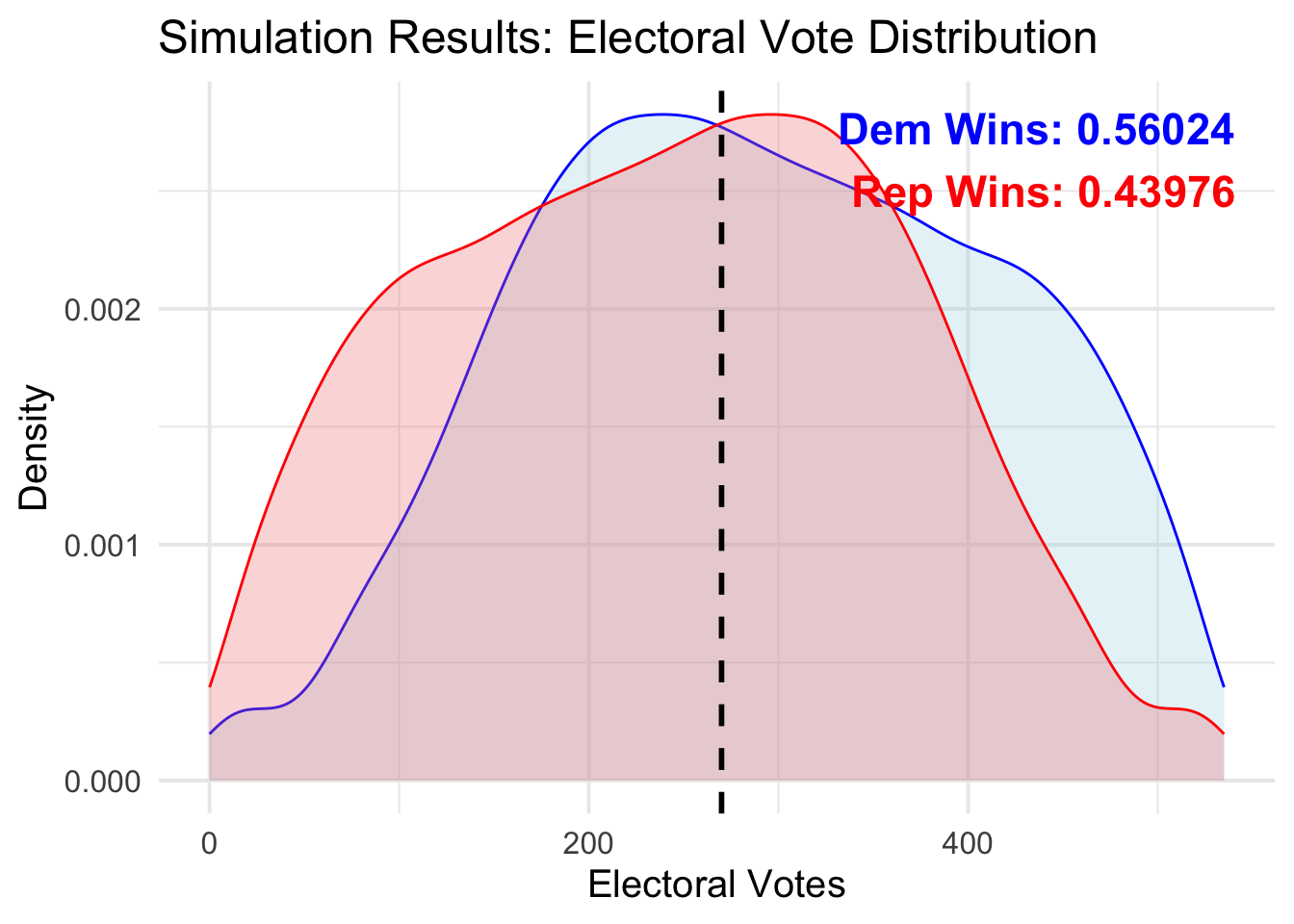 Harris wins approximately
 \(56\) percent of the time; Trump wins approximately \(44\) percent of the time. Interestingly, the most frequent individual result actually occurs when Harris wins approximately 230 electoral votes — a Democratic loss. This is, of course, balanced out by the fact that there is a large bulge of outcomes where Harris wins over 400 electoral votes.
Clearly, from this graph, you can see how large the variances are. My prior is that it is hard to imagine an election result where Harris wins over 400 votes, but this simulation says it’s possible.